Classification Problem

Binary Classification Problem

y is either 0 or 1.

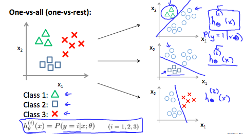
Multiclass Classification Problem

y is from 0 to n.

• Train a logistic regression classifier $$h_\theta(x)$$ for each class to predict the probability that $$y = i$$

• To make a prediction on a new $$x$$, pick the class that maximizes $$h_\theta(x)$$

• Choose 1 class, lump all the others into a single second class

• Do this repeatedly, applying binary logistic regression to each case
• Use the hypothesis that returned the highest value as our prediction

$$ y \in {0...n}\ h\theta^{(i)}(x) = P(y = i|x; \theta)\ prediction = \max_i(h\theta^{(i)}(x))

$$

Logistic Regression

• Problem with linear regression
  • Doesn't make sense for $$h_\theta(x)$$ to be > 1 or < 0

• Solution

  • Logistic/sigmoid function: fit $$h_\theta(x)$$ in between 0 & 1

    • $$ h\theta(x) = g(\theta_Tx) = g(z) = \frac{1}{1+e^{-z}}\ h\theta(x) = P(y=1|x;\theta) = 1 - P(y=0|x;\theta) $$

    • 

    • Gives probability that the output is 1

Decision Boundary

The line separating the area where y = 0 and y = 1. It is created by our hypothesis function.

$$ z \ge 0 \rightarrow h\theta(x) \ge 0.5 \rightarrow 1\ z \lt 0 \rightarrow h\theta(x) \lt 0.5 \rightarrow 0

$$

Cost Function

Original cost function for linear regression (i.e. squared-error) cannot be applied, since it does not produce a convex function with no local minima.

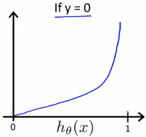
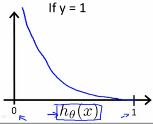
Negative Logarithmic Function

Always convex.

$$ \begin{align}

J(\theta) &= \frac{1}{m}\sum^m{i=1}Cost(h\theta(x^{(i)}), y^{(i)})\ Cost(h\theta(x), y) &= -log(h\theta(x)) &\text{ if } y = 1\ &= -log(1 - h_\theta(x)) &\text{ if } y = 0

\end{align}

$$

$$ \begin{align}

Cost(h\theta(x), y) &= 1 &\text{ if } h\theta(x) = y\ &\rightarrow \inf &\text{ if } h_\theta(x) \rightarrow (1-y) \text{ where } y = 0, 1

\end{align}

$$

Simplified

$$ Cost(h\theta(x), y) = -y log(h\theta(x)) - (1-y)log(1-h\theta(x))\ J(\theta) = \frac{1}{m}\sum^m{i=1}[-y^{(i)} log(h\theta(x^{(i)})) - (1-y^{(i)})log(1-h\theta(x^{(i)}))]

$$

Vectorized

$$ h = g(X\theta)\ J(\theta) = \frac{1}{m}[-y^T log(h) - (1-y)^Tlog(1-h)]

$$

Gradient Descent

Same algorithm as in linear regression.

$$ \begin{align}

&\text{Repeat: {}\ &\hspace{1cm}\thetaj := \theta_j - \alpha\frac{1}{m} \sum^{m}{i=1}{((h_\theta(x^{(i)}) - y^{(i)})x_j^{(i)})}\ &\text{}}

\end{align}

$$

Vectorized

$$ \begin{align}

&\text{Repeat: {}\ &\hspace{1cm}\theta_j := \theta_j - \alpha\frac{1}{m} X^T(g(X\theta)-\vec{y})\ &}

\end{align}

$$

Advanced Optimization

• Conjugate gradient
• BFGS
• L-BFGS

Implementation

1. Provide $$J(\theta)$$ & $$\frac{\partial}{\partial \theta_j}J(\theta)$$

    function [jVal, gradient] = costFunction(theta)
        jVal = [...code to compute J(theta)...];
        gradient = [...code to compute derivative of J(theta)...];
    end
   

2. Use the provided optimization algorithm fminunc with option creating function optimset

    options = optimset('GradObj', 'on', 'MaxIter', 100);
    initialTheta = zeros(2,1);
    [optTheta, functionVal, exitFlag] = fminunc(@costFunction, initialTheta, options);