Model Representation

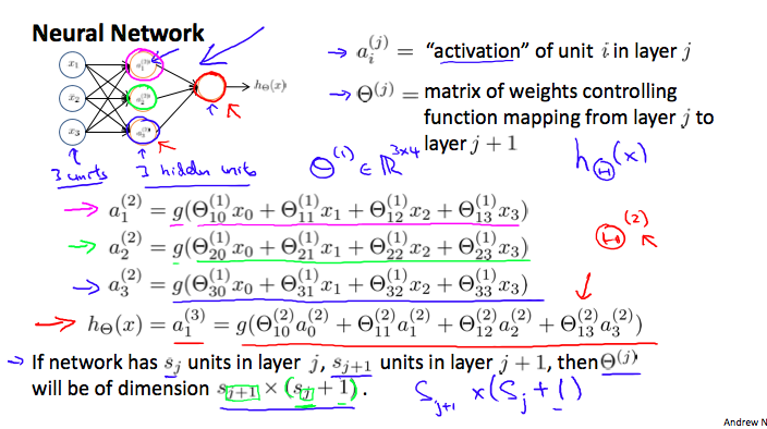
Example

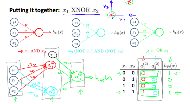
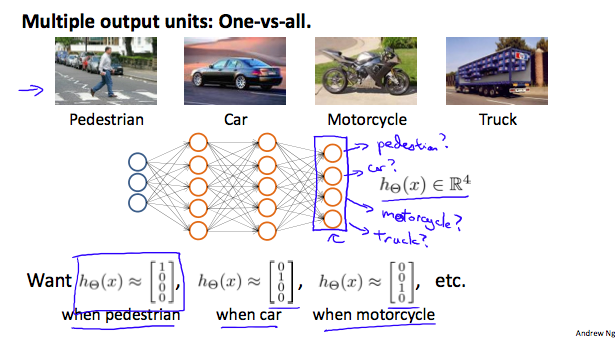
Multiclass Classification

Cost Funtion

$$J(\theta) = -\frac{1}{m}\sum^m{i=1}\sum^K{k=1}[-yk^{(i)} log(h\theta(x^{(i)}))k - (1-y_k^{(i)})log(1-h\theta(x^{(i)}))k] + \frac{\lambda}{2m} \sum^{L-1}{l=1} \sum^{sl}{i=1} \sum^{s{l+1}}{j=1} (\theta^{(l)}_{i, j})^2$$-

• Main: sum over all output nodes
• Regularization: adds up the squares of all the individual Θs in the entire network

Backpropagation

Algorithm in neural networks to minimize the cost function.

$$ min_{\theta} J(\theta)

$$

i.e. trying to find the partial derivative:

$$ \frac{\partial}{\partial \theta_{i, j}^{(l)}} J(\theta)

$$

Algorithm

1. Randomly initialize the weights
2. Implement forward propagation to get $$h_{\theta}(x^{(i)})$$ for any $$x^{(i)}$$
3. Use gradient descent or a built-in optimization function to minimize the cost function with the weights in theta
4. Implement the cost function
5. Use gradient checking to confirm that your backpropagation works
6. Disable gradient checking
7. Implement backpropagation to compute partial derivatives
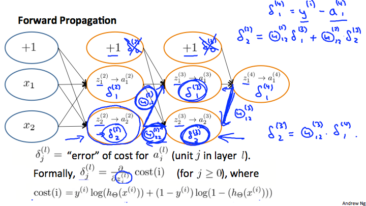
   1. Compute errors $$\delta^{(l)}_{j} = \frac{\partial}{\partial z^{(l)}_j} cost(t)$$ of each node
      1. $$cost(t) = y^{(t)} log(h\theta(x^{(t)})) + (1-y^{(t)})log(1-h\theta(x^{(t)}))$$

Training Set

$${(x^{1}, y^{1}), ..., (x^{m}, y^{m})}$$$${(x^{(1)}, y^{(1)}), ..., (x^{(m)}, y^{(m)})}$$

Steps

1. Set $$\Delta^{(l)}_{i, j} := 0$$ for all $$i, j, l$$

2. For training example t = 1 to m:

   1. Set $$a^{(1)} = x^{(t)}$$

   2. For forward layers l = 1 to L:

   3. $$a^{(l)}$$ = forward propagation
      

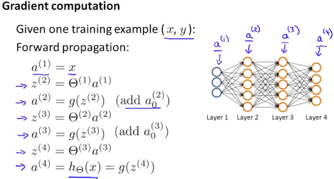
   4. Compute $$\delta^{(L)} = a^{(L)} - y^{(t)}$$

   5. For backward layers l = L-1 to 2:

      1. $$\delta^{(l)} = (\theta^{(l)})^T \delta^{(l+1)} \odot g'(z^{(l)})$$ , $$g'(z^{(l)}) = a^{(l)} \odot (1 - a^{(l)})$$

   6. $$\Delta^{(l)}{i, j} := \Delta^{(l)}{i, j} + \delta^{(l+1)} (a^{(l)})^T$$

3. Accumulator

$$ \begin{aligned} D^{(l)}{i, j} &:= \frac{1}{m} (\Delta^{(l)}{i, j} + \lambda \theta^{(l)}{i, j}) &\text{ if } j \ne 0\ &:= \frac{1}{m} (\Delta^{(l)}{i, j}) &\text{ if } j = 0\ \frac{\partial}{\partial \theta^{(l)}{i, j}} J(\theta) &:= D^{(l)}{i, j} \end{aligned}

$$

Implementation

Gradient Checking

$$ \frac{\partial}{\partial \theta} J(\theta) \approx \frac{J(\theta + \epsilon) - J(\theta - \epsilon)}{2\epsilon}\ \frac{\partial}{\partial \theta_j} J(\theta) \approx \frac{J(\theta_1, ..., \theta_j + \epsilon, ..., \theta_n) - J(\theta_1, ..., \theta_j - \epsilon, ..., \theta_n)}{2\epsilon}

$$

Check if $$deltaVector \approx gradApprox$$.

Random Initialization

Initialize $$\theta^{(l)}_{i, j}$$ to a random value within $$[-\epsilon, \epsilon]$$.

Good choice of $$\epsilon = \frac{\sqrt{6}}{\sqrt{L{in} + L{out}}}$$ where $$L{in} = s_l$$ and $$L{out} = s_{l+1}$$

Architecture

• Number of input units = dimension of features $$x^{(i)}$$
• Number of output units = number of classes
• Number of hidden units per layer = usually more the better (must balance with cost of computation as it increases with more hidden units)
• Defaults: 1 hidden layer. If more than 1, it is recommended to have the same number of units in every hidden layer